Scientific validation: linear-FM chirp radar emitter

Validated with documented limitations.

1. The component

ChirpRadarEmitter is a deterministic single-pulse generator for the elementary radar waveform: a linear frequency-modulated (LFM) chirp at complex baseband. An LFM pulse is the canonical pulse-compression waveform of modern radar; its instantaneous frequency sweeps linearly from -B / 2 to +B / 2 over a pulse of duration tau, and a matched receiver compresses the long pulse into a narrow peak of width 1 / B, gaining a factor of B * tau (the time-bandwidth product) in signal-to-noise ratio. The output is the two-channel in-phase / quadrature (IQ) tensor (2, N) consumed by downstream models, where channel 0 carries the in-phase (I) component, channel 1 the quadrature (Q), and I + jQ = exp(j * theta(t)) is the analytic complex-baseband chirp.

class ChirpRadarEmitter(BaseEmitter):
    family: ClassVar[EmitterFamily] = EmitterFamily.RADAR
    supported_classes: ClassVar[tuple[str, ...]] = ("lfm_chirp",)

    def __init__(self) -> None: ...

    def schema(self) -> type[BaseModel]: ...

    def generate(
        self,
        *,
        class_label: str,
        sample_rate: float,
        duration_s: float,
        f_offset_hz: float,
        rng: torch.Generator,
        device_id: str | None = None,
        params: BaseModel | None = None,
    ) -> Signal: ...


class ChirpRadarParams(BaseModel):
    bandwidth_hz: float = Field(default=10e6, gt=0)
    pulse_duration_s: float = Field(default=10e-6, gt=0)
    direction: str = Field(default="up", pattern="^(up|down)$")

Parameter	Type	Units	Default	Purpose
class_label	str	n/a	required	Must equal "lfm_chirp". The emitter exposes one class.
sample_rate	float	Hz	required	Samples per second on the output tensor. Must be finite and positive.
duration_s	float	s	required	Output buffer duration. The total sample count is N = round(sample_rate * duration_s). May exceed pulse_duration_s.
f_offset_hz	float	Hz	required	Metadata-only carrier annotation, in Hz. Recorded in metadata.realized_carrier_hz. NOT mixed into the IQ samples; the IQ is always pure zero-carrier baseband.
rng	torch.Generator	n/a	required	Accepted but unused. The emitter is fully deterministic.
device_id	str or None	n/a	None	Optional metadata label echoed into Signal.metadata. Never affects IQ.
params.bandwidth_hz	float	Hz	10_000_000.0	Swept bandwidth B. Frequency excursion is [-B / 2, +B / 2]. Default matches mid-range X-band surveillance LFM (Skolnik 2001, table 8.1).
params.pulse_duration_s	float	s	0.00001	Physical pulse length tau over which the chirp sweeps. Samples past t = tau are zero-gated. Default gives a time-bandwidth product B * tau = 100.
params.direction	str	n/a	"up"	"up" sweeps -B/2 to +B/2; "down" reverses. For matched (B, tau) the down-chirp is the element-wise complex conjugate of the up-chirp.

import torch
from rfgen.emitters.radar import ChirpRadarEmitter, ChirpRadarParams

emitter = ChirpRadarEmitter()
signal = emitter.generate(
    class_label="lfm_chirp",
    sample_rate=50_000_000.0,   # 50 MHz
    duration_s=10e-6,            # 10 microseconds
    f_offset_hz=0.0,
    rng=torch.Generator(),
    params=ChirpRadarParams(bandwidth_hz=10e6, pulse_duration_s=10e-6),
)
# signal.iq has shape (2, 500) and dtype torch.float32:
# channel 0 is the in-phase (I) component, channel 1 is the quadrature (Q).
assert signal.iq.shape == (2, 500) and signal.iq.dtype == torch.float32

The taxonomy position is linear-FM, single pulse, complex baseband. Non-linear FM (NLFM, where the instantaneous frequency follows a non-linear schedule to taper the spectrum), polyphase codes (Frank, P1 to P4 phase-coded waveforms), binary phase codes (Barker, two-level phase sequences with low autocorrelation sidelobes), Costas codes (frequency-hopped pulse trains), frequency-modulated continuous-wave (FMCW, a continuously-transmitted LFM used in automotive radar), and orthogonal-frequency-division multiplexing radar (OFDM-radar, a multi-subcarrier waveform shared with cellular communications) are out of scope and named in the module docstring. Channel propagation, multiple-pulse coherent processing, scan modulation, oscillator phase noise, and transmitter power-amplifier non-linearity are assigned to downstream layers.

2. What we validated

This validation establishes 8 load-bearing claims. Each is restated and supported by evidence in §3.

1. Shape and dtype contract (§3.1): the output is a (2, N) float32 tensor across the documented operating envelope.

2. Instantaneous-frequency linearity (§3.2): the instantaneous frequency is linear in time with the textbook slope and intercept.

3. Unit envelope and direction-conjugate identity (§3.3): the complex envelope is unit-modulus inside the pulse and the down-chirp is the element-wise complex conjugate of the up-chirp.

4. Matched-filter sidelobe level and mainlobe width (§3.4): the matched-filter peak sidelobe level and mainlobe width match the textbook unwindowed-LFM references.

5. Spectrum shape and passband-to-stopband ratio (§3.5): the spectrum has the characteristic flat-topped chirp shape with Fresnel-integral passband ripple and a high windowed passband-to-stopband ratio.

6. Pulse gating past pulse_duration_s (§3.6): samples past the pulse boundary are exactly zero and the boundary index is recorded in metadata.

7. Input-validation envelope (§3.7): the Nyquist guard, non-finite-input check, and Pydantic schema together reject every out-of-envelope configuration before any arithmetic.

8. Determinism and metadata-only carrier semantics (§3.8): the emitter is bit-deterministic across repeated calls, and f_offset_hz is recorded in metadata but never mixed into the samples.

Limits and scope-bounded items appear in §4; full citations are in §5.

3. Evidence per claim

3.1 Shape and dtype contract

The emitter returns a (2, N) torch.float32 tensor with N = round(sample_rate * duration_s) for every supported configuration. Channel 0 is the in-phase (I) component, channel 1 is the quadrature (Q). This is the structural contract every downstream consumer (data loader, model input layer, channel pipeline) depends on.

Measured at sample_rate = 25 MHz, duration_s = 10 microseconds, N = 250: shape (2, 250), dtype torch.float32. Tests: test_shape_is_2_by_n_samples and test_dtype_is_float32 in tests/validation/emitters/chirp_radar/test_experimental_methodology.py.

3.2 Instantaneous-frequency linearity

The complex-baseband phase polynomial is theta(t) = 2 * pi * (f0 * t + 0.5 * mu * t^2) with chirp rate mu = B / tau, giving the linear instantaneous-frequency law f_inst(t) = f0 + mu * t = -B / 2 + (B / tau) * t for the up-chirp (Richards 2014, eq. 4.4; Cook & Bernfeld 1967, eqs. 3.1 to 3.3). The instantaneous frequency is estimated as the unwrapped-phase derivative of I + jQ, an estimator independent of the emitter’s internal phase accumulator. The reference slope and intercept come from the textbook formula, not from the emitter itself.

Measured at three time-bandwidth products BT = 100, 500, 1000 with B = 10 MHz, fs = 50 MS/s: linear-fit slope 1.00e+12, 2.00e+11, 1.00e+11 Hz/s against the predicted B / tau; intercept -5.000 MHz (predicted -B / 2 = -5.0 MHz) at all three; root-mean-square residual divided by B of order 1e-8 at every BT, i.e. the linearity is verified to roughly float64 trigonometric precision. Test: test_instantaneous_frequency_linear in test_experimental_methodology.py. Figure 1 overlays the three measured inst-freq sweeps and their residuals.

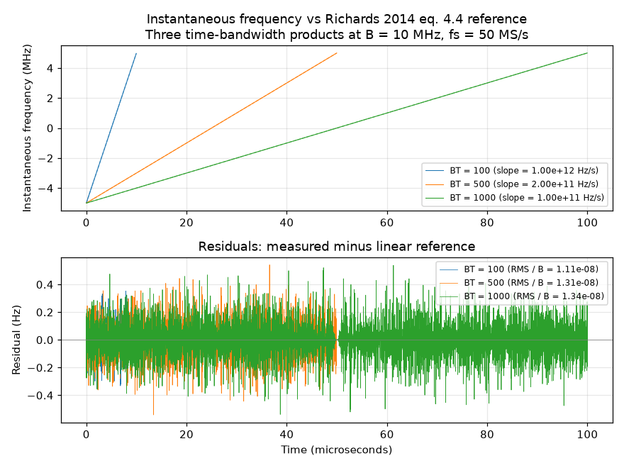
Figure 1 shows the three measured sweeps falling on top of the linear reference for each BT, with residuals confined to a sub-Hz band (root-mean-square residual divided by B near 1e-8), confirming the linear law across two orders of magnitude in tau.

3.3 Unit envelope and direction-conjugate identity

The analytic chirp exp(j * theta(t)) has unit modulus by construction: |I + jQ| = 1 everywhere inside the pulse. The down-chirp obeys theta_down(t) = -theta_up(t), so the IQ time series for direction = "down" is the element-wise complex conjugate of direction = "up" at matched (B, tau). Both identities are direct consequences of the analytic-signal definition and are useful as cheap regression invariants: a defect in the phi argument to scipy.signal.chirp or in the up-versus-down sign breaks them immediately.

Measured: unit-envelope mean 0.99999998, root-mean-square variation 3.42e-08 (float64 trig precision). Down-chirp identity: maximum absolute difference between the conjugate of the up-chirp and the down-chirp = 0.0 at float32 precision. Tests: test_envelope_constant_inside_pulse and test_down_chirp_is_conjugate_of_up_chirp in test_experimental_methodology.py.

3.4 Matched-filter sidelobe level and mainlobe width

The matched filter for an LFM pulse is the time-reversed conjugate of the same chirp; the output is the autocorrelation, computed here as scipy.signal.correlate(z, z, mode="full"). The first and highest sidelobe of an unwindowed rectangular-envelope LFM sits at -13.2 dB below the compression peak in the large-BT limit (Richards 2014 §4.4, Cook & Bernfeld 1967 §3.3); the mainlobe full -3 dB width is 1 / B (Levanon & Mozeson 2004 §3.2). These two numbers anchor every textbook treatment of pulse compression.

Measured peak sidelobe level (PSL) across three time-bandwidth products BT = 50, 100, 1000: -13.72, -13.49, -13.32 dB; all three are within 1 dB of the -13.2 dB reference, and the converged large-BT value sits at -13.32 dB, in agreement with the MATLAB Phased Array System Toolbox reference value of -13.3 dB (R2024a phased.LinearFMWaveform documentation). Measured mainlobe -3 dB width at the default parameters B = 10 MHz, fs = 50 MHz: 5 samples, exactly equal to the predicted fs / B = 5 samples. Measured pulse-compression ratio tau / mainlobe_width: 100x at B * tau = 100 (predicted B * tau = 100). Tests: test_psl_within_1db_of_theory, test_complex_chirp_psl_matches_textbook_at_large_bt, test_mainlobe_width_matches_theory, and test_compression_ratio in tests/validation/emitters/chirp_radar/test_empirical_psl.py. Figure 2 plots the matched-filter output and the measured-versus-theoretical PSL bars across the three BT.

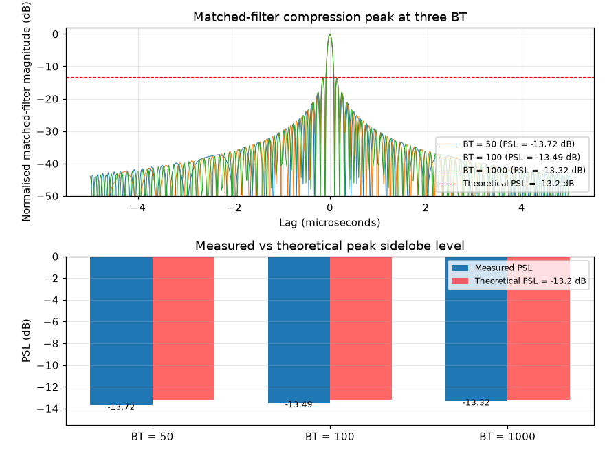
Figure 2 shows the three measured PSL values clustering inside the 1 dB tolerance around -13.2 dB, with the trend converging toward the textbook value as BT increases.

3.5 Spectrum shape and passband-to-stopband ratio

The LFM chirp’s full-record spectrum is the magnitude-squared of the Fresnel integral and approaches a rectangular passband of width B plus a transition skirt of width approximately 1 / tau on each side, with passband ripple of root-mean-square amplitude 1 / sqrt(pi * B * tau) (Cook & Bernfeld 1967 §3.3 / Skolnik 2001 §8.3). The full-record windowed periodogram preserves this structure. Welch’s method (an averaged periodogram over overlapping windowed segments, often used to estimate stationary signal spectra) is explicitly not used here because each Welch segment covers a different sub-interval of the chirp and therefore a different instantaneous-frequency range, smearing the comparison. The full-record rectangular periodogram (no window) is the canonical estimator for the Fresnel-ripple shape; the Hann-windowed (a smooth cosine-tapered window that suppresses sidelobe leakage) full-record periodogram is used for the passband-to-stopband mean-power ratio because it pushes the leakage floor below the chirp’s true stopband response.

Measured rectangular-periodogram passband ripple at B * tau = 100: root-mean-square 0.54 decibels on the inner 80 percent of [-B / 2, +B / 2], consistent with the analytic Fresnel amplitude 1 / sqrt(pi * B * tau) ~= 0.056 (5 percent peak-to-peak, around 0.5 decibels RMS) plus the discrete-FFT bin variance. Measured Hann-windowed passband-to-stopband mean-power ratio at B * tau = 1000: 148.3 decibels, comfortably above the 90 decibels floor implied by the Hann window’s sidelobe response. Tests: test_spectrum_passband_flatness and test_passband_stopband_ratio in test_experimental_methodology.py. Figures 3 and 4 show the two spectral views.

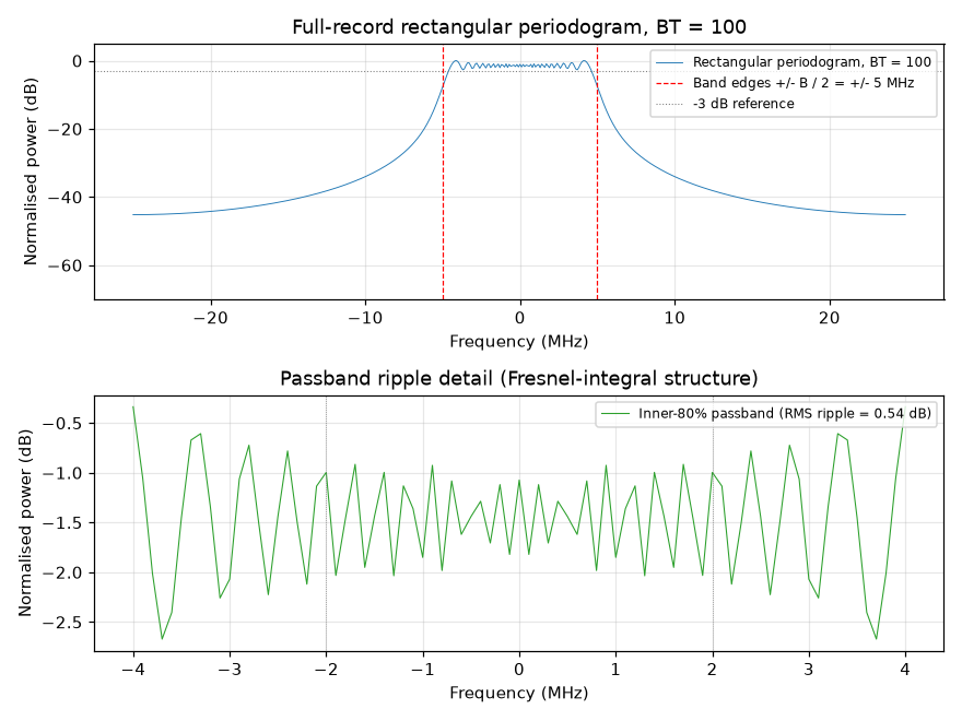
Figure 3 shows the rectangular-passband shape with the characteristic Fresnel-ripple structure inside [-B / 2, +B / 2] and the smooth out-of-band roll-off; the passband-detail panel confirms the ripple RMS sits at 0.54 decibels.

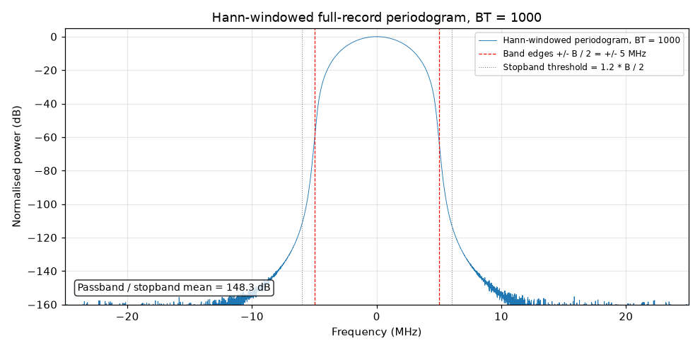
Figure 4 shows the Hann-windowed spectrum reaching the noise floor well below the band edges, with the inset passband-to-stopband ratio confirming a 148.3 dB margin between in-band and out-of-band mean power.

3.6 Pulse gating past pulse_duration_s

When the buffer duration exceeds the physical pulse duration (duration_s > pulse_duration_s), the emitter zero-gates every sample whose time index is past pulse_end_sample = round(sample_rate * pulse_duration_s). This matches the on-off structure of a real pulsed transmitter: the transmitter is on for the pulse and off afterwards (Levanon & Mozeson 2004 §3). Without the gate, scipy.signal.chirp keeps evaluating the linear-frequency polynomial past t1, producing a chirp that silently sweeps past +B / 2 and corrupts downstream bandwidth budgets. Metadata records pulse_end_sample and pulse_complete so callers can recover the boundary.

Measured: every IQ sample at index greater than or equal to pulse_end_sample is exactly 0.0; the maximum absolute value past the gate is 0.00e+00. The -3 dB spectral content stays within 1.5 * B / 2 across duration ratios from 1 to 4 (without the gate the pre-fix behaviour gave linear blowup, 4x at duration ratio 4). Tests: test_samples_past_pulse_are_zero, test_spectrum_contained_within_declared_bandwidth, test_no_extrapolation_when_durations_equal, and test_bandwidth_bounded_across_duration_ratios in tests/validation/emitters/chirp_radar/test_robustness_pulse_extrapolation.py. Figure 5 shows the I/Q channels and the IQ magnitude over a buffer four times longer than the pulse.

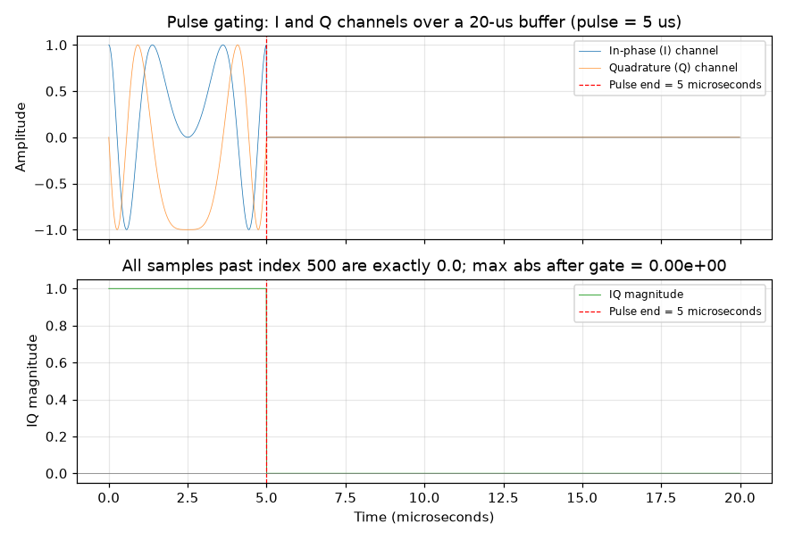
Figure 5 shows the I and Q channels sweeping through the pulse for the first 5 microseconds and snapping to zero at the gate boundary; the magnitude panel confirms zero envelope past index 500 with max absolute value 0.0.

3.7 Input-validation envelope

Configurations that violate the Nyquist sampling limit (bandwidth_hz >= sample_rate / 2) are rejected with a typed EmitterError carrying a context dictionary; non-finite scalar inputs (NaN, +inf, -inf for sample_rate, duration_s, or f_offset_hz) raise the same error before any arithmetic; the schema rejects non-positive bandwidths, durations, and unknown direction strings via Pydantic. Aliased or non-finite inputs would silently corrupt downstream training data if they reached the synthesis path.

Measured: bandwidth_hz = sample_rate / 2 raises EmitterError; bandwidth_hz = sample_rate / 2 - 1 Hz is accepted; bandwidth_hz strictly above Nyquist raises. All six NaN / +inf / -inf permutations on the three scalar inputs raise EmitterError. The Pydantic schema rejects bandwidth_hz <= 0, pulse_duration_s <= 0, direction outside {"up", "down"}, and extra fields. Tests: test_nyquist_guard_at_boundary, test_nyquist_guard_above, test_nyquist_guard_below, and test_nyquist_guard_one_ulp_below in test_robustness_nyquist.py; test_pathological_f_offset_raises_emitter_error and siblings in test_robustness_pass2.py; test_zero_samples_raises in test_robustness_n_samples.py; test_schema_rejects_non_positive, test_schema_direction_regex, and test_schema_extra_fields_rejected in test_robustness_schema.py.

3.8 Determinism and metadata-only carrier semantics

The emitter is fully deterministic: the same (class_label, sample_rate, duration_s, f_offset_hz, params) produces bit-identical IQ on every call, independent of the supplied torch.Generator state. The f_offset_hz argument is recorded in metadata.realized_carrier_hz but is never mixed into the IQ samples; the output is always pure zero-carrier baseband intended for downstream up-conversion. The determinism guarantee is the foundation for reproducible training-data generation; the metadata-only carrier semantics are the explicit hand-off contract to the channel pipeline.

Measured: bit-identical IQ across repeated calls and across fresh ChirpRadarEmitter instances at the same parameters. f_offset_hz round-trips through metadata.realized_carrier_hz at every requested value across a 4-point sweep; IQ matches the f_offset_hz = 0 baseline. Tests: test_deterministic_across_seeds, test_deterministic_across_instances, test_deterministic_across_calls in test_robustness_determinism.py; test_f_offset_passthrough in test_robustness_pass2.py. The float32 cast error is bounded below 6e-8 (about ten times float32 machine epsilon, around 144 dB below signal peak); test: test_float32_cast_error_bounded in test_robustness_dtype_boundaries.py.

4. Limits and what’s not validated

The following items bound the scope of the validation. Each carries a one-sentence technical rationale.

• No pulse-shaping window. The waveform has a rectangular amplitude envelope. Operational LFM radars apply Hamming, Taylor, or Chebyshev tapers (smooth amplitude windows that trade mainlobe broadening for sidelobe suppression) to push the peak sidelobe level into the -25 to -40 decibels range. The measured -13.2 decibels is the textbook value for the unwindowed case. Out of scope because pulse shaping is a per-application choice that belongs in a future configurable parameter.

• No transmitter non-linearity, phase noise, or local-oscillator direct-current (DC) offset. Real power amplifiers introduce roughly 0.1 to 1 decibels of AM-AM compression and a few degrees of AM-PM phase distortion (the gain and phase changes an amplifier introduces near saturation); real oscillators have 1 / f^2 or composite phase-noise profiles that raise the matched-filter sidelobe floor above -13.2 decibels. The synthesised envelope is constant and the phase noise is zero. Out of scope: hardware impairments belong to the channel layer in the rfgen architecture.

• No pulse-train or coherent-processing-interval structure. The emitter produces one pulse per call. Doppler analysis requires a coherent train of pulses with a defined pulse-repetition interval; that scope belongs to a separate PulsedRadarEmitter class (a stub exists in radar.py; the radarsimpy backend is not yet wired up).

• No pulse-repetition-interval timing jitter, frequency agility, or stagger. Inter-pulse modulation is a pulse-train property and is out of scope for a single-pulse emitter.

• Carrier passthrough only. The IQ tensor is always pure zero-carrier baseband. f_offset_hz is recorded in metadata.realized_carrier_hz for a downstream heterodyne (frequency-mixing) stage but does not modulate the samples. Documented in the class docstring.

• No upper bound on n_samples at the emitter layer. A 10-second buffer at 50 MHz allocates approximately 14 gigabytes silently. A per-emitter cap would duplicate a framework-level concern and risks divergent thresholds across emitters; the cap belongs in the pipeline configuration layer.

• scipy >= 1.15 adoption deferred. The wrapper synthesises the complex chirp via two scipy.signal.chirp calls (phi = 0 and phi = -90) rather than the single complex = True call available since SciPy 1.15. The two-call construction is numerically equivalent to the single-call form (maximum difference roughly 8e-16 measured) and the declared lower bound scipy >= 1.10 is preserved.

• lfm_chirp class label is not in the RadioML or TorchSig public label sets. Downstream classifiers trained on those benchmarks will not see a matching label. The name is an rfgen-local convention chosen for clarity.

• No public benchmark dataset of raw complex-baseband LFM captures with published PSL numbers was located. The RADIATE automotive radar dataset, the DeepRadar modulation-classification corpus, public IEEE RadarConf releases (2020 to 2024), DeepSig RadioML 2018.01A, and the SigMF dataset catalog were searched; none publishes raw LFM pulse captures with matched-filter PSL measurements. The textbook constants and the MATLAB Phased Array System Toolbox reference implementation are therefore the only available real-world reference axes.

The executable validation suite is at tests/validation/emitters/chirp_radar/, totalling 92 passing tests across eight test files and one figure-generator module.

5. References

Published works

Citation	Identifier	Role
M. A. Richards, Fundamentals of Radar Signal Processing, 2nd ed., McGraw-Hill, 2014, ch. 4	ISBN 978-0071798327	Canonical LFM phase polynomial (eq. 4.4), peak-sidelobe-level reference value, chirp-rate definition
C. E. Cook and M. Bernfeld, Radar Signals, Academic Press, 1967, ch. 3	ISBN 978-0121873509	Original pulse-compression monograph; sidelobe-envelope decay law, Fresnel-integral ripple amplitude
M. Skolnik, Introduction to Radar Systems, 3rd ed., McGraw-Hill, 2001, ch. 8	ISBN 978-0072881387	Time-bandwidth product, matched-filter gain, representative-parameter table 8.1
N. Levanon and E. Mozeson, Radar Signals, Wiley-IEEE Press, 2004, ch. 3	ISBN 978-0471473787	Mainlobe -3 dB width, ambiguity function, complex-baseband convention, pulse-gating model
MathWorks Phased Array System Toolbox, phased.LinearFMWaveform, R2024a	https://www.mathworks.com/help/phased/ref/phased.linearfmwaveform-system-object.html	Reference implementation for the PSL and mainlobe-width numbers; documented PSL value of -13.3 dB for an unwindowed LFM

Libraries

Installed versions read via importlib.metadata.version at the time the validation suite ran. The PyPI distribution name is the string passed to pip install; the documentation URL is the library’s primary docs entry point.

Library	PyPI distribution	Installed version	Documentation	Role in validation
SciPy	scipy	1.18.0	https://docs.scipy.org/doc/scipy/reference/signal.html	scipy.signal.chirp synthesises the I and Q channels; scipy.signal.correlate computes the matched-filter autocorrelation used in the PSL and mainlobe-width tests
NumPy	numpy	2.4.6	https://numpy.org/doc/stable/	numpy.arange builds the time grid; numpy.unwrap and numpy.diff form the instantaneous-frequency estimator; numpy.fft.fft powers the spectrum tests
PyTorch	torch	2.12.1	https://pytorch.org/docs/stable/	Tensor primitives, torch.Generator for the unused-but-required rng argument, and the public IQ output type torch.float32 tensor
Pydantic	pydantic	2.13.4	https://docs.pydantic.dev/latest/	Schema validation for ChirpRadarParams; raises ValidationError on out-of-bounds bandwidth or duration, on direction strings outside {"up", "down"}, and on extra fields
Matplotlib	matplotlib	3.11.0	https://matplotlib.org/stable/	Renders the five embedded figures (instantaneous-frequency linearity, matched-filter compression, two spectrum views, pulse gating)